
Building the best time-series model for electricity demand
Forecasting electricity demand is a critical task undertaken by grid operators around the world. With Banyan, we set out to build the best time-series model for this task. In a year of testing against 10 other forecasting approaches, including frontier time-series foundation models, Banyan had the lowest error in all 7 US ISOs.
Across the seven regional systems, its average error was nearly 25% lower than the closest competitor.
Two-day forecast error across seven ISO systems
The importance of forecasting electricity
Grid operators must decide how much electricity to have ready before homes and businesses need it. They use demand forecasts to schedule generators, arrange power purchases, and prepare for peaks. If demand comes in higher than expected, they may have to find extra supply at short notice. If it comes in lower, they may have paid to start generators they did not need.
Inaccurate forecasting can have serious consequences. During Winter Storm Elliott in December 2022, the Tennessee Valley Authority ordered rolling outages on December 23 and 24 as demand exceeded forecasts and generating units failed. In Nashville, neighborhoods lost power for about 10 minutes every 90 minutes to two hours during the rotations. Around 72,000 people in Nashville Electric Service’s territory were without power at the storm’s peak. The subsequent FERC and NERC inquiry found that many operators across the affected region had underestimated peak demand.
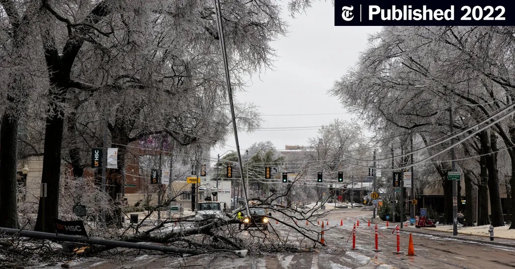
Downed utility lines and ice-covered trees after a February 2022 winter storm in Tennessee. Photo: Brad Vest/Getty Images. Source: The New York Times.
Testing a full year of electricity demand
We tested Banyan against 10 other forecasting approaches, including frontier time-series foundation models, from October 2025 through September 2026. Every six hours, each predicted demand for each of the next 48 hours. The test covered the seven U.S. regional grid systems and 80 zones within them. We scored the predictions against each operator’s published demand, collected through Grid Status.
We ran the test as though each forecast were being made at the time. Models received the weather forecasts and demand readings that would have been available then. We kept the test year out of model training and scored every approach on the same forecast hours.
Across all 87 areas, Banyan’s average error was 2.47%, compared with 2.73% for fine-tuned Timestral and 3.21% for fine-tuned Chronos-2. TiDE, an MLP-based model and the strongest model trained from scratch for the comparison, scored 3.25%. Banyan beat TiDE in every area. We measured each area’s error relative to its total demand, then averaged those scores with equal weight for each area.
Forecast error by model
Average WAPE across the 7 regional systems. Lower is better.


Figure 2. All 11 models. Select the seven regional systems, 80 zones, or all 87 areas. WAPE measures absolute forecast error relative to demand. Each area receives equal weight.
Banyan leads across regions, seasons, and forecast horizons
Banyan had the lowest average error in every month of the test year. Across all 87 areas, it also led at every forecast horizon from two to 48 hours ahead. At 48 hours, its error was 2.73%, compared with 3.11% for fine-tuned Timestral. For the seven regional systems alone, Banyan led from three to 48 hours ahead.
Forecast error on each regional system
Figure 3. System-wide error in each region. Banyan, fine-tuned Timestral, and TiDE are shown. Banyan ranks first among all 11 models on each system.
Forecasting during extreme weather periods
A forecast’s performance during extreme weather matters because demand can rise sharply while supply is under pressure. Extreme heat and cold can change demand quickly as heating and cooling systems run harder. Testing these periods shows whether a model remains accurate when operators have less room for error. In PJM’s January 20–27, 2026 cold spell, Banyan’s error was 1.15%, compared with 1.46% for fine-tuned Timestral and 2.43% for TiDE. The chart shows actual demand and predictions made roughly a day earlier.
January 20–27, 2026. The upper panel shows demand in gigawatts. The lower panel shows forecast error. Shading identifies days flagged for cold weather.
How we built Banyan
Banyan is a transformer-based model built for electricity demand forecasting. We train it across multiple grid regions, then fine-tune it for individual areas. Its training also includes auxiliary pre-training tasks.
Electricity demand depends on where people live and what the weather is doing there. A heat wave over a city can drive much more air-conditioning use than the same heat over open land. Averaging the weather across a large region can hide that difference.
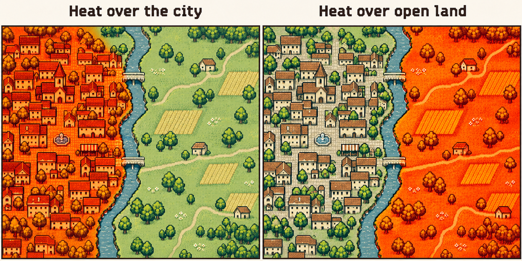
Heat over a city and heat over open land can produce different electricity demand even when the regional average temperature is the same. Conceptual illustration.
Banyan uses weather maps to retain those local differences. It combines them with past electricity demand, population, terrain, and installed solar and wind capacity to predict demand hour by hour. The results above show that this approach can outperform general-purpose time-series models, including versions fine-tuned on electricity data, on this benchmark.
Important research contributions
- Spatial inputs for electricity demand: Banyan combines weather maps with population, terrain, and installed solar and wind capacity. This gives the model information about where weather occurs and the electricity system it affects.
- A year-long evaluation under realistic operating conditions: We tested forecasts across seven regional systems and 80 zones using the information available when each forecast would have been issued. The evaluation includes seasonal changes, cold spells, and peak-demand periods.
- A direct comparison with adapted foundation models: We evaluated Timestral, Chronos-2, and TimesFM 3 both as released and after fine-tuning on electricity data. Fine-tuning reduced Timestral’s average error from 3.84% to 2.73%, making it Banyan’s closest competitor. Banyan led across all seven regional systems and in 77 of 87 areas even after competing models had learned from electricity data.
Appendix: How we trained the models and measured error
We used January 2019 through September 2024 for training and the following year for validation. Banyan was fitted through September 2025. The fine-tuned foundation models trained through September 2024, with the following year used to choose a checkpoint. After validation, the models trained from scratch were refitted through September 2025. Every model stayed fixed during the test year.
The foundation models, TFT, and DAG received load history, area-average weather, and calendar inputs. TiDE and LightGBM used weather from 184 stations. Banyan used weather maps and geographic inputs. This benchmark compares the complete approaches. Establishing how much of Banyan’s lead comes from each input or modeling choice will require additional experiments.
We issued forecasts at 00, 06, 12, and 18 UTC for the next 48 hours. We used the latest available ECMWF AIFS weather forecast and respected each area’s demand-reporting delay, which ranged from one to 61 hours. Each approach was scored on 6,052,976 matched forecast hours.
We report weighted absolute percentage error (WAPE). For each area, we divided the sum of absolute forecast errors by total observed demand. We then averaged the area scores equally. The seven-system score gives each regional system equal weight. The 87-area score gives a zone the same weight as a regional system.
Full results by model and grid area
Explore the benchmark tables
All 11 approaches · average WAPE (%)
| Model | All 87 areas | 7 ISO systems | 80 zones | Error vs Banyan | Best in (areas) |
|---|---|---|---|---|---|
| Banyan | 2.47 ● | 1.44 ● | 2.57 ● | — | 77 |
| Timestral 209M, fine-tunedMistral foundation model | 2.73 | 1.91 | 2.81 | +10 % | 9 |
| Chronos-2 120M, fine-tunedAmazon foundation model | 3.21 | 2.27 | 3.30 | +30 % | 1 |
| TiDEGoogle, 2023 | 3.25 | 2.16 | 3.35 | +31 % | 0 |
| TFTGoogle, 2019 | 3.65 | 2.62 | 3.74 | +47 % | 0 |
| TimesFM 3 331M, fine-tunedGoogle foundation model | 3.76 | 2.76 | 3.85 | +52 % | 0 |
| TimesFM 3 331M, zero-shotGoogle foundation model | 3.79 | 2.69 | 3.89 | +53 % | 0 |
| Timestral 209M, zero-shotMistral foundation model | 3.84 | 2.63 | 3.94 | +55 % | 0 |
| LightGBMgradient boosting | 4.38 | 3.65 | 4.44 | +77 % | 0 |
| Chronos-2 120M, zero-shotAmazon foundation model | 4.59 | 3.14 | 4.72 | +86 % | 0 |
| DAGICML 2026 | 4.62 | 3.30 | 4.73 | +87 % | 0 |
All 87 areas · WAPE (%) by model
FT means fine-tuned on our data. ZS means zero-shot. A dot marks the lowest error using the underlying scores before rounding.
CAISO
| Area | Banyan | Timestral FT | Chronos-2 FT | TimesFM 3 FT |
|---|---|---|---|---|
| CAISO system | 2.17 ● | 2.32 | 2.52 | 3.03 |
| PG&E | 2.28 ● | 2.54 | 2.78 | 3.39 |
| San Diego Gas & Electric | 5.29 | 5.05 ● | 5.21 | 5.90 |
| Southern California Edison | 3.30 | 3.22 ● | 3.45 | 3.95 |
| Valley Electric | 4.02 ● | 4.53 | 5.09 | 5.76 |
| Area | Timestral ZS | Chronos-2 ZS | TimesFM 3 ZS | MLP-based model (TiDE) |
|---|---|---|---|---|
| CAISO system | 2.76 | 2.91 | 2.80 | 2.72 |
| PG&E | 3.03 | 3.25 | 3.07 | 2.81 |
| San Diego Gas & Electric | 5.50 | 5.64 | 5.53 | 5.82 |
| Southern California Edison | 3.62 | 3.89 | 3.73 | 3.70 |
| Valley Electric | 5.39 | 5.94 | 5.43 | 5.21 |
| Area | TFT | DAG | LightGBM |
|---|---|---|---|
| CAISO system | 3.55 | 3.17 | 4.18 |
| PG&E | 2.96 | 3.28 | 3.45 |
| San Diego Gas & Electric | 6.95 | 6.01 | 7.62 |
| Southern California Edison | 4.51 | 4.19 | 5.67 |
| Valley Electric | 6.56 | 6.92 | 6.12 |
ERCOT
| Area | Banyan | Timestral FT | Chronos-2 FT | TimesFM 3 FT |
|---|---|---|---|---|
| ERCOT system | 1.36 ● | 1.50 | 1.79 | 1.76 |
| Coast | 2.00 ● | 2.11 | 2.43 | 2.51 |
| East | 3.36 ● | 3.57 | 4.03 | 4.10 |
| Far West | 2.99 | 2.75 | 2.75 ● | 3.13 |
| Houston load zone | 2.00 ● | 2.11 | 2.43 | 2.51 |
| North | 5.32 | 4.72 ● | 4.86 | 5.16 |
| North Central | 2.13 ● | 2.30 | 2.82 | 2.80 |
| North load zone | 1.98 ● | 2.11 | 2.61 | 2.61 |
| South | 2.28 ● | 2.33 | 2.60 | 2.65 |
| South Central | 1.96 ● | 2.14 | 2.57 | 2.69 |
| South load zone | 1.61 ● | 1.73 | 2.06 | 2.16 |
| West | 6.34 | 5.51 ● | 5.96 | 6.33 |
| West load zone | 2.40 | 2.20 ● | 2.23 | 2.64 |
| Area | Timestral ZS | Chronos-2 ZS | TimesFM 3 ZS | MLP-based model (TiDE) |
|---|---|---|---|---|
| ERCOT system | 2.01 | 2.69 | 1.98 | 1.81 |
| Coast | 2.68 | 3.34 | 2.65 | 2.37 |
| East | 4.44 | 5.48 | 4.44 | 4.16 |
| Far West | 2.79 | 2.87 | 2.83 | 3.45 |
| Houston load zone | 2.68 | 3.33 | 2.65 | 2.37 |
| North | 4.98 | 5.16 | 5.05 | 5.66 |
| North Central | 3.20 | 4.28 | 3.11 | 2.53 |
| North load zone | 3.00 | 4.05 | 2.93 | 2.32 |
| South | 2.81 | 3.36 | 2.77 | 2.56 |
| South Central | 2.96 | 3.96 | 2.93 | 2.40 |
| South load zone | 2.41 | 3.26 | 2.35 | 1.85 |
| West | 6.08 | 6.56 | 6.10 | 7.56 |
| West load zone | 2.29 | 2.41 | 2.34 | 2.77 |
| Area | TFT | DAG | LightGBM |
|---|---|---|---|
| ERCOT system | 1.76 | 3.22 | 3.05 |
| Coast | 2.52 | 3.12 | 3.74 |
| East | 4.78 | 6.25 | 5.40 |
| Far West | 3.04 | 3.12 | 3.35 |
| Houston load zone | 2.52 | 3.11 | 3.74 |
| North | 5.95 | 6.36 | 6.24 |
| North Central | 2.91 | 5.31 | 5.63 |
| North load zone | 2.62 | 4.89 | 5.17 |
| South | 2.89 | 3.44 | 4.43 |
| South Central | 2.96 | 4.29 | 4.76 |
| South load zone | 2.42 | 3.33 | 4.17 |
| West | 6.75 | 9.52 | 7.96 |
| West load zone | 2.55 | 2.81 | 2.76 |
ISO-NE
| Area | Banyan | Timestral FT | Chronos-2 FT | TimesFM 3 FT |
|---|---|---|---|---|
| ISO-NE system | 1.93 ● | 2.71 | 3.25 | 4.28 |
| Connecticut | 2.41 ● | 2.79 | 3.57 | 4.47 |
| Maine | 2.80 ● | 3.82 | 4.50 | 6.06 |
| New Hampshire | 2.09 ● | 2.47 | 3.14 | 4.20 |
| Northeast Mass. | 1.81 ● | 2.26 | 2.92 | 3.67 |
| Rhode Island | 3.63 ● | 3.79 | 4.40 | 5.18 |
| Southeast Mass. | 2.92 ● | 3.46 | 4.22 | 5.24 |
| Vermont | 4.19 ● | 4.93 | 5.71 | 7.77 |
| Western/Central Mass. | 2.45 ● | 2.98 | 3.65 | 4.69 |
| Area | Timestral ZS | Chronos-2 ZS | TimesFM 3 ZS | MLP-based model (TiDE) |
|---|---|---|---|---|
| ISO-NE system | 4.12 | 4.60 | 4.12 | 2.82 |
| Connecticut | 5.14 | 6.29 | 4.92 | 3.60 |
| Maine | 5.95 | 6.06 | 5.82 | 4.29 |
| New Hampshire | 4.27 | 5.36 | 4.38 | 3.10 |
| Northeast Mass. | 4.06 | 4.90 | 3.73 | 3.04 |
| Rhode Island | 5.66 | 6.85 | 5.67 | 4.95 |
| Southeast Mass. | 5.56 | 6.59 | 5.26 | 4.21 |
| Vermont | 6.98 | 7.30 | 7.10 | 5.37 |
| Western/Central Mass. | 5.25 | 6.14 | 5.23 | 3.46 |
| Area | TFT | DAG | LightGBM |
|---|---|---|---|
| ISO-NE system | 3.60 | 4.86 | 4.25 |
| Connecticut | 3.32 | 5.60 | 4.29 |
| Maine | 5.40 | 6.38 | 5.35 |
| New Hampshire | 2.98 | 4.44 | 3.73 |
| Northeast Mass. | 3.20 | 4.46 | 3.33 |
| Rhode Island | 5.58 | 6.70 | 5.06 |
| Southeast Mass. | 4.62 | 5.98 | 4.75 |
| Vermont | 6.54 | 7.45 | 6.50 |
| Western/Central Mass. | 4.24 | 5.07 | 3.86 |
MISO
| Area | Banyan | Timestral FT | Chronos-2 FT | TimesFM 3 FT |
|---|---|---|---|---|
| MISO system | 0.93 ● | 1.70 | 1.99 | 2.44 |
| Zone 1 | 1.75 ● | 2.48 | 2.94 | 3.55 |
| Zone 4 | 2.20 ● | 2.50 | 3.00 | 3.79 |
| Zone 6 | 1.91 ● | 2.07 | 2.59 | 3.39 |
| Zones 2 and 7 | 1.33 ● | 2.83 | 3.44 | 4.28 |
| Zones 3 and 5 | 1.54 ● | 2.43 | 2.89 | 3.41 |
| Zones 8, 9, and 10 | 1.66 ● | 2.39 | 2.74 | 2.86 |
| Area | Timestral ZS | Chronos-2 ZS | TimesFM 3 ZS | MLP-based model (TiDE) |
|---|---|---|---|---|
| MISO system | 2.19 | 2.60 | 2.35 | 1.90 |
| Zone 1 | 3.78 | 4.08 | 3.76 | 3.13 |
| Zone 4 | 4.56 | 5.23 | 4.21 | 3.29 |
| Zone 6 | 3.46 | 4.62 | 3.58 | 2.75 |
| Zones 2 and 7 | 4.00 | 4.34 | 4.23 | 2.76 |
| Zones 3 and 5 | 3.83 | 4.88 | 3.84 | 2.80 |
| Zones 8, 9, and 10 | 3.16 | 4.59 | 3.25 | 3.43 |
| Area | TFT | DAG | LightGBM |
|---|---|---|---|
| MISO system | 2.17 | 2.53 | 2.62 |
| Zone 1 | 3.13 | 3.56 | 4.42 |
| Zone 4 | 3.77 | 4.96 | 5.80 |
| Zone 6 | 3.37 | 3.97 | 3.46 |
| Zones 2 and 7 | 3.56 | 4.05 | 3.01 |
| Zones 3 and 5 | 3.21 | 4.20 | 4.55 |
| Zones 8, 9, and 10 | 3.71 | 5.11 | 4.87 |
NYISO
| Area | Banyan | Timestral FT | Chronos-2 FT | TimesFM 3 FT |
|---|---|---|---|---|
| NYISO system | 1.45 ● | 2.09 | 2.50 | 3.27 |
| Capital | 2.97 ● | 3.30 | 3.79 | 4.78 |
| Central | 2.90 ● | 3.07 | 3.50 | 4.43 |
| Dunwoodie | 2.35 ● | 2.59 | 3.09 | 3.73 |
| Genesee | 2.69 ● | 2.96 | 3.45 | 4.56 |
| Hudson Valley | 2.76 ● | 3.23 | 3.80 | 4.64 |
| Long Island | 2.50 ● | 3.13 | 3.92 | 4.86 |
| Millwood | 3.96 ● | 4.09 | 4.69 | 5.36 |
| Mohawk Valley | 4.02 ● | 4.17 | 4.64 | 6.06 |
| New York City | 1.42 ● | 1.72 | 2.17 | 2.64 |
| North | 3.43 | 3.31 ● | 3.42 | 3.98 |
| West | 2.33 ● | 2.34 | 2.71 | 3.46 |
| Area | Timestral ZS | Chronos-2 ZS | TimesFM 3 ZS | MLP-based model (TiDE) |
|---|---|---|---|---|
| NYISO system | 3.01 | 3.45 | 3.10 | 2.07 |
| Capital | 4.58 | 4.86 | 4.56 | 3.81 |
| Central | 4.26 | 4.51 | 4.24 | 3.88 |
| Dunwoodie | 3.86 | 4.37 | 3.60 | 3.39 |
| Genesee | 4.24 | 4.60 | 4.24 | 3.47 |
| Hudson Valley | 4.62 | 5.32 | 4.65 | 3.53 |
| Long Island | 4.31 | 4.74 | 4.31 | 3.28 |
| Millwood | 5.41 | 6.21 | 5.23 | 4.97 |
| Mohawk Valley | 5.50 | 5.68 | 5.40 | 4.99 |
| New York City | 2.56 | 3.25 | 2.57 | 1.87 |
| North | 3.67 | 3.59 | 3.55 | 3.91 |
| West | 3.02 | 3.30 | 3.02 | 2.95 |
| Area | TFT | DAG | LightGBM |
|---|---|---|---|
| NYISO system | 2.80 | 3.57 | 3.22 |
| Capital | 4.78 | 5.53 | 5.13 |
| Central | 4.25 | 5.33 | 5.07 |
| Dunwoodie | 3.88 | 4.51 | 3.87 |
| Genesee | 3.59 | 4.96 | 4.40 |
| Hudson Valley | 4.26 | 5.37 | 5.14 |
| Long Island | 3.93 | 5.58 | 4.36 |
| Millwood | 5.37 | 6.19 | 6.24 |
| Mohawk Valley | 5.28 | 6.46 | 6.55 |
| New York City | 2.22 | 3.12 | 2.63 |
| North | 4.25 | 4.39 | 4.44 |
| West | 3.22 | 3.79 | 4.26 |
PJM
| Area | Banyan | Timestral FT | Chronos-2 FT | TimesFM 3 FT |
|---|---|---|---|---|
| PJM system | 1.06 ● | 1.38 | 1.82 | 2.29 |
| AEP | 1.27 ● | 1.44 | 1.82 | 2.27 |
| ATSI | 1.64 ● | 1.78 | 2.24 | 2.73 |
| Allegheny Power | 1.60 ● | 1.86 | 2.37 | 2.77 |
| Atlantic Electric | 3.02 ● | 3.44 | 3.98 | 4.82 |
| BGE | 2.34 ● | 2.54 | 3.15 | 3.60 |
| ComEd | 2.00 ● | 2.15 | 2.60 | 3.25 |
| Dayton | 1.93 ● | 2.12 | 2.69 | 3.40 |
| Delmarva | 2.35 ● | 2.84 | 3.51 | 4.00 |
| Dominion | 1.35 ● | 1.64 | 2.03 | 2.19 |
| Duke Ohio/Kentucky | 2.06 ● | 2.20 | 2.77 | 3.25 |
| Duquesne | 2.10 ● | 2.22 | 2.52 | 2.98 |
| East Kentucky | 4.16 ● | 4.51 | 4.90 | 5.39 |
| JCP&L | 2.66 ● | 3.01 | 3.61 | 4.32 |
| Met-Ed | 1.81 ● | 2.08 | 2.70 | 3.27 |
| Mid-Atlantic region | 1.57 ● | 1.87 | 2.46 | 2.98 |
| PECO | 1.95 ● | 2.11 | 2.63 | 3.06 |
| PPL | 1.70 ● | 1.83 | 2.40 | 2.84 |
| PSE&G | 2.13 ● | 2.39 | 2.96 | 3.68 |
| Penelec | 1.58 ● | 1.72 | 2.19 | 2.86 |
| Pepco | 2.29 ● | 2.58 | 3.11 | 3.71 |
| Rockland Electric | 2.42 ● | 2.66 | 3.18 | 3.86 |
| Western region | 1.13 ● | 1.33 | 1.78 | 2.30 |
| Area | Timestral ZS | Chronos-2 ZS | TimesFM 3 ZS | MLP-based model (TiDE) |
|---|---|---|---|---|
| PJM system | 2.11 | 2.95 | 2.20 | 1.93 |
| AEP | 2.18 | 2.80 | 2.28 | 1.72 |
| ATSI | 2.64 | 3.24 | 2.76 | 2.24 |
| Allegheny Power | 2.79 | 3.61 | 2.85 | 2.03 |
| Atlantic Electric | 4.56 | 5.66 | 4.57 | 3.85 |
| BGE | 3.83 | 4.96 | 3.62 | 2.96 |
| ComEd | 3.22 | 3.97 | 3.26 | 2.67 |
| Dayton | 3.22 | 4.04 | 3.36 | 2.72 |
| Delmarva | 3.99 | 5.26 | 3.80 | 2.85 |
| Dominion | 2.38 | 3.37 | 2.27 | 1.84 |
| Duke Ohio/Kentucky | 3.38 | 4.27 | 3.31 | 2.64 |
| Duquesne | 3.07 | 3.87 | 3.09 | 2.76 |
| East Kentucky | 5.45 | 6.41 | 5.31 | 4.84 |
| JCP&L | 4.42 | 5.27 | 4.41 | 3.16 |
| Met-Ed | 3.16 | 3.97 | 3.32 | 2.46 |
| Mid-Atlantic region | 2.96 | 3.94 | 2.99 | 2.17 |
| PECO | 3.14 | 4.10 | 3.16 | 2.46 |
| PPL | 2.81 | 3.65 | 2.94 | 2.25 |
| PSE&G | 3.73 | 4.38 | 3.69 | 2.65 |
| Penelec | 2.42 | 3.03 | 2.69 | 2.10 |
| Pepco | 3.98 | 4.99 | 3.64 | 2.89 |
| Rockland Electric | 3.70 | 4.53 | 3.85 | 2.98 |
| Western region | 2.14 | 2.86 | 2.29 | 1.85 |
| Area | TFT | DAG | LightGBM |
|---|---|---|---|
| PJM system | 2.14 | 2.84 | 3.65 |
| AEP | 1.89 | 3.46 | 5.25 |
| ATSI | 2.28 | 3.42 | 2.80 |
| Allegheny Power | 2.48 | 3.37 | 2.83 |
| Atlantic Electric | 5.17 | 5.80 | 4.45 |
| BGE | 3.54 | 4.44 | 3.69 |
| ComEd | 2.99 | 4.02 | 3.49 |
| Dayton | 2.97 | 3.80 | 3.22 |
| Delmarva | 3.89 | 5.03 | 3.72 |
| Dominion | 2.25 | 3.28 | 4.42 |
| Duke Ohio/Kentucky | 3.06 | 3.99 | 3.03 |
| Duquesne | 2.79 | 3.54 | 3.21 |
| East Kentucky | 5.04 | 5.98 | 5.72 |
| JCP&L | 3.75 | 5.01 | 4.17 |
| Met-Ed | 3.21 | 3.73 | 2.89 |
| Mid-Atlantic region | 2.79 | 3.77 | 2.76 |
| PECO | 2.82 | 3.74 | 2.96 |
| PPL | 2.90 | 3.63 | 2.81 |
| PSE&G | 3.13 | 4.40 | 3.58 |
| Penelec | 2.29 | 3.01 | 2.51 |
| Pepco | 3.76 | 4.47 | 3.69 |
| Rockland Electric | 3.70 | 4.35 | 3.79 |
| Western region | 1.91 | 2.97 | 3.59 |
SPP
| Area | Banyan | Timestral FT | Chronos-2 FT | TimesFM 3 FT |
|---|---|---|---|---|
| SPP system | 1.17 ● | 1.67 | 2.03 | 2.26 |
| AEP West | 1.97 ● | 2.22 | 2.78 | 3.02 |
| City of Springfield | 2.82 ● | 3.07 | 3.72 | 4.15 |
| Empire District | 2.92 ● | 3.17 | 4.02 | 4.44 |
| Evergy Kansas Central | 1.95 ● | 2.18 | 2.77 | 3.15 |
| Evergy Metro | 2.79 ● | 2.99 | 3.53 | 4.10 |
| Evergy Missouri West | 3.08 ● | 3.73 | 4.59 | 4.92 |
| Grand River Dam Auth. | 1.85 | 1.77 ● | 1.99 | 2.06 |
| Independence P&L | 3.82 ● | 3.97 | 4.61 | 5.01 |
| Kansas City BPU | 3.04 ● | 3.12 | 3.74 | 4.51 |
| Lincoln Electric | 3.57 | 3.49 ● | 4.20 | 4.54 |
| Nebraska PPD | 4.76 ● | 5.41 | 6.15 | 6.84 |
| OG&E | 2.46 ● | 2.58 | 3.06 | 3.24 |
| Omaha PPD | 3.40 | 2.98 ● | 3.52 | 3.88 |
| Southwestern Public Service | 1.65 ● | 1.96 | 2.18 | 2.34 |
| Sunflower Electric | 2.74 ● | 2.98 | 3.33 | 3.55 |
| WAPA Upper Great Plains | 1.60 ● | 1.86 | 2.05 | 2.27 |
| Western Farmers | 2.44 ● | 2.58 | 3.00 | 3.27 |
| Area | Timestral ZS | Chronos-2 ZS | TimesFM 3 ZS | MLP-based model (TiDE) |
|---|---|---|---|---|
| SPP system | 2.24 | 2.77 | 2.31 | 1.87 |
| AEP West | 3.54 | 4.98 | 3.43 | 2.70 |
| City of Springfield | 4.93 | 6.03 | 4.62 | 4.01 |
| Empire District | 5.08 | 6.67 | 4.85 | 4.55 |
| Evergy Kansas Central | 3.66 | 4.72 | 3.55 | 2.84 |
| Evergy Metro | 4.82 | 5.93 | 4.32 | 3.97 |
| Evergy Missouri West | 5.90 | 7.32 | 5.26 | 4.31 |
| Grand River Dam Auth. | 2.35 | 2.76 | 2.28 | 2.59 |
| Independence P&L | 5.41 | 7.48 | 5.30 | 4.73 |
| Kansas City BPU | 4.67 | 5.96 | 4.74 | 4.16 |
| Lincoln Electric | 5.26 | 7.02 | 4.99 | 4.66 |
| Nebraska PPD | 6.93 | 7.99 | 6.73 | 5.50 |
| OG&E | 3.84 | 4.55 | 3.55 | 2.91 |
| Omaha PPD | 4.23 | 5.44 | 4.08 | 3.67 |
| Southwestern Public Service | 2.36 | 2.59 | 2.30 | 2.18 |
| Sunflower Electric | 3.75 | 4.05 | 3.66 | 3.47 |
| WAPA Upper Great Plains | 2.57 | 2.82 | 2.46 | 2.54 |
| Western Farmers | 3.25 | 4.63 | 3.33 | 3.19 |
| Area | TFT | DAG | LightGBM |
|---|---|---|---|
| SPP system | 2.29 | 2.95 | 4.59 |
| AEP West | 3.35 | 3.92 | 3.61 |
| City of Springfield | 4.18 | 5.56 | 4.78 |
| Empire District | 5.73 | 5.86 | 5.93 |
| Evergy Kansas Central | 2.97 | 4.08 | 2.91 |
| Evergy Metro | 4.81 | 6.04 | 5.26 |
| Evergy Missouri West | 4.89 | 5.89 | 5.02 |
| Grand River Dam Auth. | 2.20 | 6.31 | 4.34 |
| Independence P&L | 4.76 | 6.24 | 4.95 |
| Kansas City BPU | 4.56 | 5.40 | 4.93 |
| Lincoln Electric | 4.15 | 5.56 | 7.83 |
| Nebraska PPD | 6.18 | 7.92 | 6.53 |
| OG&E | 3.10 | 4.86 | 6.39 |
| Omaha PPD | 3.81 | 4.69 | 5.42 |
| Southwestern Public Service | 2.06 | 2.40 | 2.57 |
| Sunflower Electric | 3.36 | 3.74 | 4.74 |
| WAPA Upper Great Plains | 2.81 | 3.51 | 2.87 |
| Western Farmers | 3.08 | 4.35 | 3.51 |
Model references
- Timestral — Mistral’s time-series foundation models.
- Chronos-2 — Amazon’s Chronos forecasting models.
- TimesFM 3 — Google Research’s TimesFM models.
- TiDE — Long-term Forecasting with TiDE: Time-series Dense Encoder.
- TFT — Temporal Fusion Transformers for Interpretable Multi-horizon Time Series Forecasting.
- LightGBM — Microsoft Research’s LightGBM project.
- DAG — A Dual Correlation Network for Time Series Forecasting with Exogenous Variables.